Chapter 7, Thematic Mapping

For this assignment, we had to pick a type of thematic map, and create data for the poverty levels in the United States.  I chose quantile mapping, because I found it to be the most aesthetically appealing, while still displaying accurate data (!!NOTE!! Louisiana does not have data, and I could not find an efficient and accurate way to enter it, so all values in that area are set to zero).

As you can see, the areas with the most poverty are mostly in the south, with a small patch in the northern USA.  Why did I pick this map?  While the alternatives did add more accurate detail, they made for a cluttered and messy overview, especially when you take into account that the data was separated by counties.  However, one problem I experienced with quantile mapping was that it seemed to be incompatible with Alaska and Hawaii...  This type of mapping did not appear to register with them, and failed to produce any results.

Despite the problems, I actually find that this map is very effective.  I went about creating it by first using kriging to organize and group the data, then, I went about and transformed that data into a more visually appealing map.  This was accomplished by using the Geostatistical Analyst tool, the Geostatistical Wizard, and properly entering the data.

Chapter 6 Maps

Here are the maps that I created for our chapter 6 assignment.  The information and processes that went behind their creation can be found in my post "Chapter 5 and 6 Essays".

A normal QQ Plot, derived from USGS earthquake data.

Covariance (top) and semivariance (bottom) graphs.

Trend Analysis Chart, from same source.  Notice how it has the rough outline of the United States (source material).

A Voronoi Map, same source.  Again, see if you can make out the rough outline of the USA.

Chapter 5 and 6 Essays

I forgot to post my essay for chapter 5, so I thought I would combine the two into one post and save some time.

Chapter 5

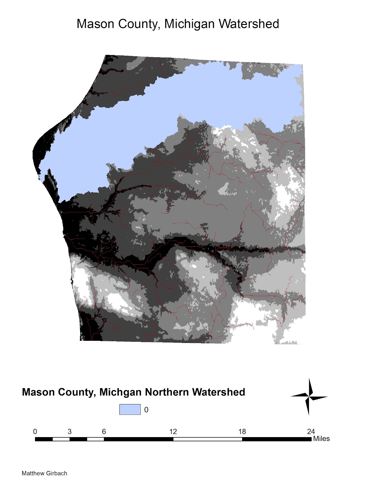
                Using the information gathered with the three maps (IDW, Kriging, and Spline), I have determined that the highest values of fecal coliform levels reside in the northern part of the study area.  The IDW and spline maps show that the levels have the highest concentration in the very northernmost tip, whilst the kriging map shows that they are most prominent in the northwest portion of the map.  By examining all three and comparing them, I was able to average out the three sets of data and come to my conclusion that the fecal coliform levels are mostly present in the northern area of the map, mainly in the northernmost area, with a smaller concentration in the middle of the map.

Chapter 6

                In this assignment, we had to take earthquake data from the USGS and create points on our map, by taking the data from an Excel file we were to create.  Using this data, I was able to find out that the west coast of the United States had approximately 4960 earthquakes, and the east coast had approximately 529, from the period of January 1^st 2010 to February 1^st 2012.  I was able to create many charts and maps, detailing both depth and magnitude (these will be posted to my blog and to the EMU website.  However, using the information, I was able to find that the center of the earthquakes (the point in the middle of each set of data) was in the northeast portion of Nevada.

                Using a normal QQ Plot, I was able to find that the magnitude of these earthquakes was fairly consistent and “normal” in a mathematical sense.  Most points were able to be plotted normally along a straight line, with very little variance at the ends (there were a few points that were at the extremes of each end).  The most powerful was recorded at a magnitude of 18, and appeared to be near Virginia.  This occurred on 4/24/2011.  In the end, I was very surprised by how many earthquakes were on the east coast, and that the most powerful one was as well.

Lesson 5 Assignments

For this assignment, we had to create various maps utilizing different types of data interpolation for fecal coliform levels.  In this case, we used spline, IDW, and kriging to achieve our goals.  Below are my three maps utilizing these techniques.

IDW Map

Kriging Map

Spline Map

Lesson 4

This is my map for lesson 4.  Here is the paper I wrote describing it:

For this lab, I used the Little Colorado River dataset.  To find it, I looked it up on Google Maps, and then found the approximate location on the USGS Seamless Server.  To derive the sediment transport index, I used a variety of steps which we learned in class.  What follows is a summary of what I did.  First, I unzipped the DEM and loaded it into ArcGIS.  Then, I took the DEM and converted it from the GCS North America 1983 geographic coordinate system into the USA Contiguous Albers Equal Area projected coordinate system.

                After inserting the new map into a new dataframe, I filled the sinks and created a new raster from that data.  Then, I created Flow Accumulation and Direction maps.  Next, I used the raster calculator to find streams with a value greater than that of 3000.  After using this data to create a stream network map, I used the stream to feature function to create a vector map from the stream link data.

                Then, I created a pour point at the beginning of the Little Colorado River, and calculated a watershed like I did in Lesson 3.  I also did the operations to calculate sediment deposition.  When creating my map, I had a great deal of difficulty including the sediment data into the map.  I couldn’t fit the entire stream data into my map, so I included the watershed of the area, and a legend with the Sediment Deposition per Square Meter.  I apologize if this isn’t exactly what was asked for, and I can make changes if needed.

Adventures in ArcGIS! Watersheds

For this assignment, we had to construct a watershed chart for a specific area.  I chose Mason county in Michigan.  First, I went to the Seamless Server and downloaded a DEM of the county, and converted it to the proper measurements for ArcGIS.  Then, went through various processes, including creating a pour point.  The steps I took can be found within the Model Builder Model, which I will include below.  This assignment went smoothly, and I encountered few problems overall.

Stream Network of Mason County, including all streams with a value greater than 3000.

Watershed of northern stream network in Mason County.  Notice the pour point, where the watershed meets Lake Michigan in the farthest left side of the map.

The Model Builder Model.  This details the steps I took to create the Watershed Map.

Washtenaw and Wayne Maps

Note from Matt: It seems that Blogger has failed to properly post my maps.  Way to go, site!  In lieu of the lost maps, I will attempt to recreate the post with the best of my memory (however shoddy it may be).

The following maps are based on various filters available in ArcGIS.

TIN Map

Aspect Map

Hill Curve Map

Hillshade Map

Slope Map

For this map, we needed to find suitable locations for a vinyard in California, given specific criteria.  Keep in mind that while this map does in fact detail the necessary criteria for the information given, it does not account for land which is already owned, etc.