Lesson 4

This is my map for lesson 4.  Here is the paper I wrote describing it:

For this lab, I used the Little Colorado River dataset.  To find it, I looked it up on Google Maps, and then found the approximate location on the USGS Seamless Server.  To derive the sediment transport index, I used a variety of steps which we learned in class.  What follows is a summary of what I did.  First, I unzipped the DEM and loaded it into ArcGIS.  Then, I took the DEM and converted it from the GCS North America 1983 geographic coordinate system into the USA Contiguous Albers Equal Area projected coordinate system.

                After inserting the new map into a new dataframe, I filled the sinks and created a new raster from that data.  Then, I created Flow Accumulation and Direction maps.  Next, I used the raster calculator to find streams with a value greater than that of 3000.  After using this data to create a stream network map, I used the stream to feature function to create a vector map from the stream link data.

                Then, I created a pour point at the beginning of the Little Colorado River, and calculated a watershed like I did in Lesson 3.  I also did the operations to calculate sediment deposition.  When creating my map, I had a great deal of difficulty including the sediment data into the map.  I couldn’t fit the entire stream data into my map, so I included the watershed of the area, and a legend with the Sediment Deposition per Square Meter.  I apologize if this isn’t exactly what was asked for, and I can make changes if needed.

Adventures in ArcGIS! Watersheds

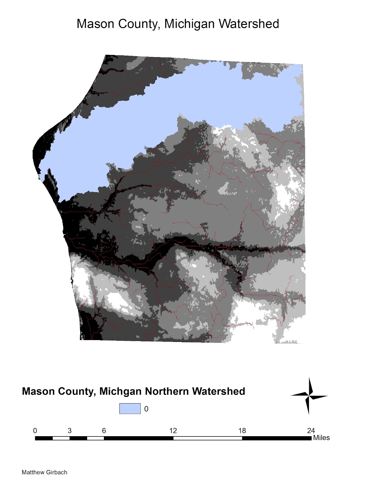
For this assignment, we had to construct a watershed chart for a specific area.  I chose Mason county in Michigan.  First, I went to the Seamless Server and downloaded a DEM of the county, and converted it to the proper measurements for ArcGIS.  Then, went through various processes, including creating a pour point.  The steps I took can be found within the Model Builder Model, which I will include below.  This assignment went smoothly, and I encountered few problems overall.

Stream Network of Mason County, including all streams with a value greater than 3000.

Watershed of northern stream network in Mason County.  Notice the pour point, where the watershed meets Lake Michigan in the farthest left side of the map.

The Model Builder Model.  This details the steps I took to create the Watershed Map.

Washtenaw and Wayne Maps

Note from Matt: It seems that Blogger has failed to properly post my maps.  Way to go, site!  In lieu of the lost maps, I will attempt to recreate the post with the best of my memory (however shoddy it may be).

The following maps are based on various filters available in ArcGIS.

TIN Map

Aspect Map

Hill Curve Map

Hillshade Map

Slope Map

For this map, we needed to find suitable locations for a vinyard in California, given specific criteria.  Keep in mind that while this map does in fact detail the necessary criteria for the information given, it does not account for land which is already owned, etc.

Adventures in ArcGIS! Part 1

Today, I experimented in the art of creating 3D models in ArcGIS 10.  More specifically, I worked on getting my 3D maps to display different kinds of data, such as slope models.  Speaking of which, I was able to create a 3D slope model of Washtenaw and Wayne counties in Michigan:

With this model, the red areas are those of sharper slope, while the green areas are those of gentler slope.  To make this map, I first downloaded digital elevation model data from michigan.gov/cgi, and loaded it into ArcMap.  I then mosaic'ed the rasters together, making sure I used the Focal Mean tool to eliminate any seams in the image.  After that, I converted the raster to a TIN file, and loaded the file in ArcScene.  After doing that, I converted the DEM file I created earlier into slope data, and draped it over the TIN, creating the image you see above.  I have also done work with draping orthophotos over this TIN as well:

This is the Manchester area, as viewed when draped upon the aforementioned TIN file.  This picture constitutes the NW, NE, SW, and SE areas of the village.

 Here is a hillshade map, using the slope raster.

 This is an aspect map, showing which direction each hill faces.

And a curvature map.